Minor topics in CNN – 다중클래스 분류, fastai metric 사용

강의영상

https://youtube.com/playlist?list=PLQqh36zP38-wVdrvMFFtAcAM2QC7ZpnN3

imports

import torch 
import torchvision
import numpy as np
from fastai.vision.all import *

import graphviz
def gv(s): return graphviz.Source('digraph G{ rankdir="LR"'+s + '; }');

CNN 다중클래스 분류

결론 (그냥 외우세요)

- 2개의 class를 구분하는 문제가 아니라 \(k\)개의 class를 구분해야 한다면?

일반적인 개념

손실함수: BCE loss \(\to\) Cross Entropy loss
마지막층의 선형변환: torch.nn.Linear(?,1) \(\to\) torch.nn.Linear(?,k)
마지막층의 활성화: sig \(\to\) softmax

파이토치 한정

y의형태: (n,) vector + int형 // (n,k) one-hot encoded vector + float형
손실함수: torch.nn.BCEWithLogitsLoss, \(\to\) torch.nn.CrossEntropyLoss
마지막층의 선형변환: torch.nn.Linear(?,1) \(\to\) torch.nn.Linear(?,k)
마지막층의 활성화: None \(\to\) None (손실함수에 이미 마지막층의 활성화가 포함)

실습: 3개의 클래스를 구분

path = untar_data(URLs.MNIST)

training set

X0 = torch.stack([torchvision.io.read_image(str(fname)) for fname in (path/'training/0').ls()])
X1 = torch.stack([torchvision.io.read_image(str(fname)) for fname in (path/'training/1').ls()])
X2 = torch.stack([torchvision.io.read_image(str(fname)) for fname in (path/'training/2').ls()])
X = torch.concat([X0,X1,X2])/255
y = torch.tensor([0]*len(X0) + [1]*len(X1)+ [2]*len(X2))#.reshape(-1,1)

test set

X0 = torch.stack([torchvision.io.read_image(str(fname)) for fname in (path/'testing/0').ls()])
X1 = torch.stack([torchvision.io.read_image(str(fname)) for fname in (path/'testing/1').ls()])
X2 = torch.stack([torchvision.io.read_image(str(fname)) for fname in (path/'testing/2').ls()])
XX = torch.concat([X0,X1,X2])/255
yy = torch.tensor([0]*len(X0) + [1]*len(X1)+ [2]*len(X2))#.reshape(-1,1)

(1) dls

len(X)

ds1 = torch.utils.data.TensorDataset(X,y) 
ds2 = torch.utils.data.TensorDataset(XX,yy) 
dl1 = torch.utils.data.DataLoader(ds1,batch_size=1862) # 에폭당 11번 iter
dl2 = torch.utils.data.DataLoader(ds2,batch_size=3147) # 
dls = DataLoaders(dl1,dl2)

(2) lrnr

net1 = torch.nn.Sequential(
    torch.nn.Conv2d(1,16,(5,5)),
    torch.nn.ReLU(),
    torch.nn.MaxPool2d((2,2)),
    torch.nn.Flatten()
)

net1(X).shape

torch.Size([18623, 2304])

net = torch.nn.Sequential(
    net1,
    torch.nn.Linear(2304,3) # 0,1,2 3개를 구분하는 문제이므로 out_features=3 
)
loss_fn = torch.nn.CrossEntropyLoss()

lrnr = Learner(dls,net,loss_fn)

(3) 학습

lrnr.fit(10)

epoch	train_loss	valid_loss	time
0	0.155762	0.045966	00:00
1	0.087853	0.093116	00:00
2	0.089215	0.033146	00:00
3	0.075707	0.039687	00:00
4	0.063615	0.031188	00:00
5	0.055850	0.029167	00:00
6	0.050883	0.028610	00:00
7	0.047144	0.028127	00:00
8	0.044129	0.027425	00:00
9	0.041849	0.026887	00:00

(4) 예측

lrnr.model.to("cpu")

Sequential(
  (0): Sequential(
    (0): Conv2d(1, 16, kernel_size=(5, 5), stride=(1, 1))
    (1): ReLU()
    (2): MaxPool2d(kernel_size=(2, 2), stride=(2, 2), padding=0, dilation=1, ceil_mode=False)
    (3): Flatten(start_dim=1, end_dim=-1)
  )
  (1): Linear(in_features=2304, out_features=3, bias=True)
)

pd.DataFrame(lrnr.model(XX)).assign(y=yy)

	0	1	2	y
0	2.025615	-17.453382	-2.335629	0
1	2.531184	-9.890347	-3.949971	0
2	1.587324	-13.035635	-3.257438	0
3	2.749664	-9.918694	-6.867003	0
4	2.155442	-15.885134	-3.019295	0
...	...	...	...	...
3142	-9.030737	-8.673495	1.204605	2
3143	-3.569304	-10.748278	-0.645055	2
3144	-3.627095	-12.919289	1.046083	2
3145	-5.151307	-9.524368	0.068864	2
3146	-8.014889	-14.518770	2.732226	2

3147 rows × 4 columns

pd.DataFrame(lrnr.model(XX)).assign(y=yy).query('y==0')

	0	1	2	y
0	2.025615	-17.453382	-2.335629	0
1	2.531184	-9.890347	-3.949971	0
2	1.587324	-13.035635	-3.257438	0
3	2.749664	-9.918694	-6.867003	0
4	2.155442	-15.885134	-3.019295	0
...	...	...	...	...
975	4.450414	-19.329332	-5.451057	0
976	2.597144	-21.202513	-2.372313	0
977	3.089397	-15.486772	-3.171502	0
978	2.591355	-17.475590	-3.039083	0
979	4.575789	-21.636261	-5.077421	0

980 rows × 4 columns

대체적으로 첫번째 칼럼의 숫자들이 다른칼럼보다 크다.

pd.DataFrame(lrnr.model(XX)).assign(y=yy).query('y==1')

	0	1	2	y
980	-7.629252	2.701625	-3.049654	1
981	-6.666027	2.027717	-4.440878	1
982	-7.120140	3.354897	-3.937105	1
983	-7.139010	2.058928	-2.954304	1
984	-6.999043	3.258377	-3.432081	1
...	...	...	...	...
2110	-7.406105	4.032059	-3.826451	1
2111	-6.172441	3.187883	-3.490717	1
2112	-7.035848	3.202726	-3.547020	1
2113	-7.149322	1.741414	-1.765136	1
2114	-5.775263	3.041395	-2.980052	1

1135 rows × 4 columns

대체적으로 두번째 칼럼의 숫자들이 다른칼럼보다 크다.

pd.DataFrame(lrnr.model(XX)).assign(y=yy).query('y==2')

	0	1	2	y
2115	-7.452892	-7.137640	0.605079	2
2116	-5.262731	-7.798437	-1.708323	2
2117	-9.056837	-9.649239	1.557607	2
2118	-6.614496	-10.291727	1.293422	2
2119	-3.120885	-10.670292	-0.660188	2
...	...	...	...	...
3142	-9.030737	-8.673495	1.204605	2
3143	-3.569304	-10.748278	-0.645055	2
3144	-3.627095	-12.919289	1.046083	2
3145	-5.151307	-9.524368	0.068864	2
3146	-8.014889	-14.518770	2.732226	2

1032 rows × 4 columns

대체적으로 세번째 칼럼의 숫자들이 다른칼럼보다 크다.

- 예측하는방법? - 칼럼0의 숫자가 크다 -> y=0일 확률이 큼 - 칼럼1의 숫자가 크다 -> y=1일 확률이 큼 - 칼럼2의 숫자가 크다 -> y=2일 확률이 큼

공부: Softmax

- 눈치: softmax를 쓰기 직전의 숫자들은 (n,k)꼴로 되어있음. 각 observation 마다 k개의 숫자가 있는데, 그중에서 유난히 큰 하나의 숫자가 있음.

- torch.nn.Softmax() 손계산

(예시1) – 잘못계산

sftmax = torch.nn.Softmax(dim=0)

_netout = torch.tensor([[-2.0,-2.0,0.0],
                        [3.14,3.14,3.14],
                        [0.0,0.0,2.0],
                        [2.0,2.0,4.0],
                        [0.0,0.0,0.0]])
_netout

tensor([[-2.0000, -2.0000,  0.0000],
        [ 3.1400,  3.1400,  3.1400],
        [ 0.0000,  0.0000,  2.0000],
        [ 2.0000,  2.0000,  4.0000],
        [ 0.0000,  0.0000,  0.0000]])

sftmax(_netout)

tensor([[0.0041, 0.0041, 0.0115],
        [0.7081, 0.7081, 0.2653],
        [0.0306, 0.0306, 0.0848],
        [0.2265, 0.2265, 0.6269],
        [0.0306, 0.0306, 0.0115]])

(예시2) – 이게 맞게 계산되는 것임

sftmax = torch.nn.Softmax(dim=1)

_netout

tensor([[-2.0000, -2.0000,  0.0000],
        [ 3.1400,  3.1400,  3.1400],
        [ 0.0000,  0.0000,  2.0000],
        [ 2.0000,  2.0000,  4.0000],
        [ 0.0000,  0.0000,  0.0000]])

sftmax(_netout)

tensor([[0.1065, 0.1065, 0.7870],
        [0.3333, 0.3333, 0.3333],
        [0.1065, 0.1065, 0.7870],
        [0.1065, 0.1065, 0.7870],
        [0.3333, 0.3333, 0.3333]])

(예시3) – 차원을 명시안하면 맞게 계산해주고 경고 줌

sftmax = torch.nn.Softmax()

_netout

tensor([[-2.0000, -2.0000,  0.0000],
        [ 3.1400,  3.1400,  3.1400],
        [ 0.0000,  0.0000,  2.0000],
        [ 2.0000,  2.0000,  4.0000],
        [ 0.0000,  0.0000,  0.0000]])

sftmax(_netout)

/home/cgb4/anaconda3/envs/py37/lib/python3.7/site-packages/ipykernel_launcher.py:1: UserWarning: Implicit dimension choice for softmax has been deprecated. Change the call to include dim=X as an argument.
  """Entry point for launching an IPython kernel.

tensor([[0.1065, 0.1065, 0.7870],
        [0.3333, 0.3333, 0.3333],
        [0.1065, 0.1065, 0.7870],
        [0.1065, 0.1065, 0.7870],
        [0.3333, 0.3333, 0.3333]])

(예시4) – 진짜 손계산

_netout

tensor([[-2.0000, -2.0000,  0.0000],
        [ 3.1400,  3.1400,  3.1400],
        [ 0.0000,  0.0000,  2.0000],
        [ 2.0000,  2.0000,  4.0000],
        [ 0.0000,  0.0000,  0.0000]])

torch.exp(_netout)

tensor([[ 0.1353,  0.1353,  1.0000],
        [23.1039, 23.1039, 23.1039],
        [ 1.0000,  1.0000,  7.3891],
        [ 7.3891,  7.3891, 54.5981],
        [ 1.0000,  1.0000,  1.0000]])

0.1353/(0.1353 + 0.1353 + 1.0000), 0.1353/(0.1353 + 0.1353 + 1.0000), 1.0000/(0.1353 + 0.1353 + 1.0000) # 첫 obs

(0.10648512513773022, 0.10648512513773022, 0.7870297497245397)

np.exp(_netout[1])/np.exp(_netout[1]).sum() # 두번째 obs

tensor([0.3333, 0.3333, 0.3333])

np.apply_along_axis(lambda x: np.exp(x) / np.exp(x).sum(),1,_netout)

array([[0.10650698, 0.10650698, 0.78698605],
       [0.33333334, 0.33333334, 0.33333334],
       [0.10650699, 0.10650699, 0.78698605],
       [0.10650698, 0.10650698, 0.78698605],
       [0.33333334, 0.33333334, 0.33333334]], dtype=float32)

공부: CrossEntropyLoss

`#` torch.nn.CrossEntropyLoss() 손계산: one-hot version

loss_fn = torch.nn.CrossEntropyLoss()

_netout

tensor([[-2.0000, -2.0000,  0.0000],
        [ 3.1400,  3.1400,  3.1400],
        [ 0.0000,  0.0000,  2.0000],
        [ 2.0000,  2.0000,  4.0000],
        [ 0.0000,  0.0000,  0.0000]])

_y_onehot = torch.tensor([[0,0,1],
                          [0,1,0],
                          [0,0,1],
                          [0,0,1],
                          [1,0,0]])*1.0
_y_onehot

tensor([[0., 0., 1.],
        [0., 1., 0.],
        [0., 0., 1.],
        [0., 0., 1.],
        [1., 0., 0.]])

sftmax = torch.nn.Softmax(dim=1) 
sftmax(_netout), _y_onehot

(tensor([[0.1065, 0.1065, 0.7870],
         [0.3333, 0.3333, 0.3333],
         [0.1065, 0.1065, 0.7870],
         [0.1065, 0.1065, 0.7870],
         [0.3333, 0.3333, 0.3333]]),
 tensor([[0., 0., 1.],
         [0., 1., 0.],
         [0., 0., 1.],
         [0., 0., 1.],
         [1., 0., 0.]]))

- 계산결과

loss_fn(_netout,_y_onehot)

tensor(0.5832)

- torch.sum(torch.log(sftmax(_netout)) * _y_onehot)/5

tensor(0.5832)

- 계산하는 방법도 중요한데 torch.nn.CrossEntropyLoss() 에는 softmax 활성화함수가 이미 포함되어 있다는 것을 확인하는 것이 더 중요함.

- 따라서 torch.nn.CrossEntropyLoss() 는 사실 torch.nn.CEWithSoftmaxLoss() 정도로 바꾸는 것이 더 말이 되는 것 같다.

`#` torch.nn.CrossEntropyLoss() 손계산: lenght \(n\) vertor version

_netout

tensor([[-2.0000, -2.0000,  0.0000],
        [ 3.1400,  3.1400,  3.1400],
        [ 0.0000,  0.0000,  2.0000],
        [ 2.0000,  2.0000,  4.0000],
        [ 0.0000,  0.0000,  0.0000]])

_y = torch.tensor([2,1,2,2,0])

loss_fn(_netout,_y)

tensor(0.5832)

실습: \(k=2\)로 두면 이진분류도 가능

- download data

path = untar_data(URLs.MNIST)

training

X0 = torch.stack([torchvision.io.read_image(str(fname)) for fname in (path/'training/0').ls()])
X1 = torch.stack([torchvision.io.read_image(str(fname)) for fname in (path/'training/1').ls()])
X = torch.concat([X0,X1])/255
y = torch.tensor([0]*len(X0) + [1]*len(X1))#.reshape(-1,1)

y_onehot = torch.nn.functional.one_hot(y).float()
#y_onehot = torch.tensor(list(map(lambda x: [1,0] if x==0 else [0,1],y))).float()

test

X0 = torch.stack([torchvision.io.read_image(str(fname)) for fname in (path/'testing/0').ls()])
X1 = torch.stack([torchvision.io.read_image(str(fname)) for fname in (path/'testing/1').ls()])
XX = torch.concat([X0,X1])/255
yy = torch.tensor([0]*len(X0) + [1]*len(X1))#.reshape(-1,1)

yy_onehot = torch.nn.functional.one_hot(yy).float()
#yy_onehot = torch.tensor(list(map(lambda x: [1,0] if x==0 else [0,1],yy))).float()

(1) dls

ds1 = torch.utils.data.TensorDataset(X,y_onehot) 
ds2 = torch.utils.data.TensorDataset(XX,yy_onehot) 
dl1 = torch.utils.data.DataLoader(ds1,batch_size=1862) # 에폭당 11번 iter
dl2 = torch.utils.data.DataLoader(ds2,batch_size=3147) # 
dls = DataLoaders(dl1,dl2)

(2) lrnr

net = torch.nn.Sequential(
    torch.nn.Conv2d(1,16,(5,5)),
    torch.nn.ReLU(),
    torch.nn.MaxPool2d((2,2)),
    torch.nn.Flatten(),
    torch.nn.Linear(2304,2)
    #torch.nn.Softmax()
)
loss_fn = torch.nn.CrossEntropyLoss()
lrnr = Learner(dls,net,loss_fn)

(3) 학습

lrnr.fit(10)

epoch	train_loss	valid_loss	time
0	0.018623	0.012110	00:00
1	0.017453	0.010544	00:00
2	0.016391	0.009324	00:00
3	0.015412	0.008343	00:00
4	0.014506	0.007542	00:00
5	0.013664	0.006874	00:00
6	0.012881	0.006318	00:00
7	0.012152	0.005849	00:00
8	0.011473	0.005448	00:00
9	0.010841	0.005103	00:00

(4) 예측 및 시각화

lrnr.model.to("cpu")

Sequential(
  (0): Conv2d(1, 16, kernel_size=(5, 5), stride=(1, 1))
  (1): ReLU()
  (2): MaxPool2d(kernel_size=(2, 2), stride=(2, 2), padding=0, dilation=1, ceil_mode=False)
  (3): Flatten(start_dim=1, end_dim=-1)
  (4): Linear(in_features=2304, out_features=2, bias=True)
)

sftmax = torch.nn.Softmax(dim=1) 
sig = torch.nn.Sigmoid()
fig,ax = plt.subplots(1,2,figsize=(8,4))
ax[0].plot(net(X).diff(axis=1).data,',',color="C1")
ax[1].plot(y)
ax[1].plot(sftmax(net(X))[:,1].data,',')
#ax[1].plot(sig(net(X).diff(axis=1)).data,',')
fig.suptitle("Training Set",size=15)

Text(0.5, 0.98, 'Training Set')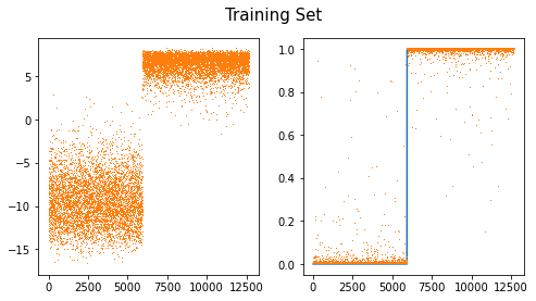

fig,ax = plt.subplots(1,2,figsize=(8,4))
ax[0].plot(net(XX).diff(axis=1).data,',',color="C1")
ax[1].plot(yy)
ax[1].plot(sftmax(net(XX))[:,1].data,',')
#ax[1].plot(sig(net(XX).diff(axis=1)).data,',')
fig.suptitle("Test Set",size=15)

Text(0.5, 0.98, 'Test Set')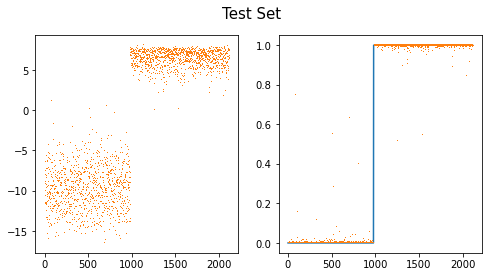

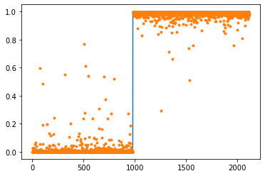
- note: softmax(u1,u2)=[sig(u1-u2), sig(u2-u1)]=[1-sig(u2-u1),sig(u2-u1)]

공부: 이진분류에서 소프트맥스 vs 시그모이드

- 이진분류문제 = “y=0 or y=1” 을 맞추는 문제 = 성공과 실패를 맞추는 문제 = 성공확률과 실패확률을 추정하는 문제

- softmax, sigmoid

softmax: (실패확률, 성공확률) 꼴로 결과가 나옴 // softmax는 실패확률과 성공확률을 둘다 추정한다.
sigmoid: (성공확률) 꼴로 결과가 나옴 // sigmoid는 성공확률만 추정한다.

- 그런데 “실패확률=1-성공확률” 이므로 사실상 둘은 같은걸 추정하는 셈이다. (성공확률만 추정하면 실패확률은 저절로 추정되니까)

- 아래는 사실상 같은 모형이다.

Code

gv('''
splines=line
subgraph cluster_1{
    style=filled;
    color=lightgrey;
    "?"
    "??"
    ".."
    "???"
    label = "Layer ?"
}
subgraph cluster_2{
    style=filled;
    color=lightgrey;
    "?" -> "node1"
    "??" -> "node1"
    ".." -> "node1"
    "???" -> "node1"
    
    "?" -> "node2"
    "??" -> "node2"
    ".." -> "node2"
    "???" -> "node2"
    
    "?" -> "..."
    "??" -> "..."
    ".." -> "..."
    "???" -> "..."
    
    "?" -> "node2304"
    "??" -> "node2304"
    ".." -> "node2304"
    "???" -> "node2304"

    label = "Layer: ReLU"
}
subgraph cluster_3{
    style=filled;
    color=lightgrey;
    "node1" -> "y1"
    "node2" -> "y1"
    "..." -> "y1"
    "node2304" -> "y1"
    
    "node1" -> "y2"
    "node2" -> "y2"
    "..." -> "y2"
    "node2304" -> "y2"    
    label = "Layer: Softmax"
}
''')

Code

gv('''
splines=line
subgraph cluster_1{
    style=filled;
    color=lightgrey;
    "?"
    "??"
    ".."
    "???"
    label = "Layer ?"
}
subgraph cluster_2{
    style=filled;
    color=lightgrey;
    "?" -> "node1"
    "??" -> "node1"
    ".." -> "node1"
    "???" -> "node1"
    
    "?" -> "node2"
    "??" -> "node2"
    ".." -> "node2"
    "???" -> "node2"
    
    "?" -> "..."
    "??" -> "..."
    ".." -> "..."
    "???" -> "..."
    
    "?" -> "node2304"
    "??" -> "node2304"
    ".." -> "node2304"
    "???" -> "node2304"

    label = "Layer: ReLU"
}
subgraph cluster_3{
    style=filled;
    color=lightgrey;
    "node1" -> "y"
    "node2" -> "y"
    "..." -> "y"
    "node2304" -> "y"
    label = "Layer: Sigmoid"
}
''')

- 둘은 사실상 같은 효과를 주는 모형인데 학습할 파라메터는 sigmoid의 경우가 더 적다. \(\to\) sigmoid를 사용하는 모형이 비용은 싸고 효과는 동일하다는 말 \(\to\) 이진분류 한정해서는 softmax를 쓰지말고 sigmoid를 써야함.

softmax가 갑자기 너무 안좋아보이는데 sigmoid는 k개의 클래스로 확장이 불가능한 반면 softmax는 확장이 용이하다는 장점이 있음

소프트맥스 vs 시그모이드 정리

- 결론

소프트맥스는 시그모이드의 확장이다.
클래스의 수가 2개일 경우에는 (Sigmoid, BCEloss) 조합을 사용해야 하고 클래스의 수가 2개보다 클 경우에는 (Softmax, CrossEntropyLoss) 를 사용해야 한다.

- 그런데 사실.. 클래스의 수가 2개일 경우일때 (Softmax, CrossEntropyLoss)를 사용해도 그렇게 큰일나는것은 아니다. (흑백이미지를 칼라잉크로 출력하는 느낌)

참고

\(y\)	분포가정	마지막층의 활성화함수	손실함수
3.45, 4.43, … (연속형)	정규분포	None (or Identity)	MSE
0 or 1	이항분포 with \(n=1\) (=베르누이)	Sigmoid	BCE
[0,0,1], [0,1,0], [1,0,0]	다항분포 with \(n=1\)	Softmax	Cross Entropy

fastai metric 사용

데이터준비

- download data

path = untar_data(URLs.MNIST)

- training set

X0 = torch.stack([torchvision.io.read_image(str(fname)) for fname in (path/'training/0').ls()])
X1 = torch.stack([torchvision.io.read_image(str(fname)) for fname in (path/'training/1').ls()])
X = torch.concat([X0,X1])/255
y = torch.tensor([0.0]*len(X0) + [1.0]*len(X1)).reshape(-1,1)

- test set

X0 = torch.stack([torchvision.io.read_image(str(fname)) for fname in (path/'testing/0').ls()])
X1 = torch.stack([torchvision.io.read_image(str(fname)) for fname in (path/'testing/1').ls()])
XX = torch.concat([X0,X1])/255
yy = torch.tensor([0.0]*len(X0) + [1.0]*len(X1)).reshape(-1,1)

X.shape,XX.shape,y.shape,yy.shape

(torch.Size([12665, 1, 28, 28]),
 torch.Size([2115, 1, 28, 28]),
 torch.Size([12665, 1]),
 torch.Size([2115, 1]))

사용자정의 메트릭이용

(1) dls 만들기

ds1 = torch.utils.data.TensorDataset(X,y)
ds2 = torch.utils.data.TensorDataset(XX,yy)
dl1 = torch.utils.data.DataLoader(ds1,batch_size=1266) 
dl2 = torch.utils.data.DataLoader(ds2,batch_size=2115) 
dls = DataLoaders(dl1,dl2)

(2) lrnr 생성

net = torch.nn.Sequential(
    torch.nn.Conv2d(1,16,(5,5)),
    torch.nn.ReLU(),
    torch.nn.MaxPool2d((2,2)),
    torch.nn.Flatten(),
    torch.nn.Linear(2304,1),
    torch.nn.Sigmoid()
)
loss_fn = torch.nn.BCELoss()

def acc(yhat,y) : 
    return ((yhat>0.5)==y).float().mean()

def err(yhat,y):
    return 1-((yhat>0.5)==y).float().mean()

lrnr = Learner(dls,net,loss_fn,metrics=[acc,err])

(3) 학습

lrnr.fit(10)

epoch	train_loss	valid_loss	acc	err	time
0	0.930635	0.633062	0.463357	0.536643	00:00
1	0.700525	0.435254	0.989125	0.010875	00:00
2	0.562099	0.293302	0.992435	0.007565	00:00
3	0.453646	0.169834	0.992908	0.007092	00:00
4	0.360984	0.098153	0.994326	0.005674	00:00
5	0.286862	0.062732	0.993853	0.006147	00:00
6	0.229778	0.044261	0.994799	0.005201	00:00
7	0.185838	0.032975	0.995745	0.004255	00:00
8	0.151484	0.025062	0.996217	0.003783	00:00
9	0.124157	0.019350	0.996690	0.003310	00:00

(4) 예측

생략

fastai지원 메트릭이용– 잘못된사용

(1) dls 만들기

ds1 = torch.utils.data.TensorDataset(X,y)
ds2 = torch.utils.data.TensorDataset(XX,yy)
dl1 = torch.utils.data.DataLoader(ds1,batch_size=1266) 
dl2 = torch.utils.data.DataLoader(ds2,batch_size=2115) 
dls = DataLoaders(dl1,dl2)

(2) lrnr 생성

net = torch.nn.Sequential(
    torch.nn.Conv2d(1,16,(5,5)),
    torch.nn.ReLU(),
    torch.nn.MaxPool2d((2,2)),
    torch.nn.Flatten(),
    torch.nn.Linear(2304,1),
    torch.nn.Sigmoid()
)
loss_fn = torch.nn.BCELoss()
lrnr = Learner(dls,net,loss_fn,metrics=[accuracy,error_rate])

accuracy??

Signature: accuracy(inp, targ, axis=-1)
Source:   
def accuracy(inp, targ, axis=-1):
    "Compute accuracy with `targ` when `pred` is bs * n_classes"
    pred,targ = flatten_check(inp.argmax(dim=axis), targ)
    return (pred == targ).float().mean()
File:      ~/anaconda3/envs/py37/lib/python3.7/site-packages/fastai/metrics.py
Type:      function

error_rate??

Signature: error_rate(inp, targ, axis=-1)
Source:   
def error_rate(inp, targ, axis=-1):
    "1 - `accuracy`"
    return 1 - accuracy(inp, targ, axis=axis)
File:      ~/anaconda3/envs/py37/lib/python3.7/site-packages/fastai/metrics.py
Type:      function

(3) 학습

lrnr.fit(10)

epoch	train_loss	valid_loss	accuracy	error_rate	time
0	0.958819	0.638672	0.463357	0.536643	00:00
1	0.698769	0.425380	0.463357	0.536643	00:00
2	0.556408	0.278437	0.463357	0.536643	00:00
3	0.447104	0.153257	0.463357	0.536643	00:00
4	0.352915	0.088516	0.463357	0.536643	00:00
5	0.278620	0.056958	0.463357	0.536643	00:00
6	0.221951	0.040489	0.463357	0.536643	00:00
7	0.178791	0.030974	0.463357	0.536643	00:00
8	0.145480	0.024886	0.463357	0.536643	00:00
9	0.119392	0.020659	0.463357	0.536643	00:00

이상하다..?

(4) 예측

lrnr.model.to("cpu")

Sequential(
  (0): Conv2d(1, 16, kernel_size=(5, 5), stride=(1, 1))
  (1): ReLU()
  (2): MaxPool2d(kernel_size=(2, 2), stride=(2, 2), padding=0, dilation=1, ceil_mode=False)
  (3): Flatten(start_dim=1, end_dim=-1)
  (4): Linear(in_features=2304, out_features=1, bias=True)
  (5): Sigmoid()
)

plt.plot(yy)
plt.plot(lrnr.model(XX).data,'.')

맞추는건 잘 맞추는데?

fastai지원 메트릭이용– 올바른 사용(1)

- 가정

X의 형태는 (n,채널,픽셀,픽셀)로 가정한다.
y의 형태는 (n,) 벡터이다. 즉 \(n\times 1\) 이 아니라 그냥 길이가 \(n\)인 벡터로 가정한다.
y의 각 원소는 0,1,2,3,… 와 같이 카테고리를 의미하는 숫자이어야 하며 이 숫자는 int형으로 저장되어야 한다.
loss function은 CrossEntropyLoss()를 쓴다고 가정한다. (따라서 네트워크의 최종레이어는 torch.nn.Linear(?,클래스의수) 꼴이 되어야 한다.)

(1) dls 만들기

y.to(torch.int64).reshape(-1),yy.to(torch.int64).reshape(-1)

(tensor([0, 0, 0,  ..., 1, 1, 1]), tensor([0, 0, 0,  ..., 1, 1, 1]))

ds1 = torch.utils.data.TensorDataset(X,y.to(torch.int64).reshape(-1))
ds2 = torch.utils.data.TensorDataset(XX,yy.to(torch.int64).reshape(-1))
dl1 = torch.utils.data.DataLoader(ds1,batch_size=1266) 
dl2 = torch.utils.data.DataLoader(ds2,batch_size=2115) 
dls = DataLoaders(dl1,dl2)

(2) lrnr 생성

net = torch.nn.Sequential(
    torch.nn.Conv2d(1,16,(5,5)),
    torch.nn.ReLU(),
    torch.nn.MaxPool2d((2,2)),
    torch.nn.Flatten(),
    torch.nn.Linear(2304,2),
)
loss_fn = torch.nn.CrossEntropyLoss()
lrnr = Learner(dls,net,loss_fn,metrics=[accuracy,error_rate])

(3) 학습

lrnr.fit(10)

epoch	train_loss	valid_loss	accuracy	error_rate	time
0	1.083689	0.592268	0.463357	0.536643	00:00
1	0.674220	0.340684	0.963593	0.036407	00:00
2	0.510727	0.152380	0.991489	0.008511	00:00
3	0.380071	0.069530	0.997163	0.002837	00:00
4	0.284898	0.038776	0.997163	0.002837	00:00
5	0.217856	0.025257	0.997163	0.002837	00:00
6	0.169902	0.018588	0.997163	0.002837	00:00
7	0.134621	0.014637	0.998582	0.001418	00:00
8	0.107967	0.012024	0.998582	0.001418	00:00
9	0.087427	0.010147	0.998582	0.001418	00:00

fastai지원 메트릭이용– 올바른 사용(2)

- 가정

X의 형태는 (n,채널,픽셀,픽셀)로 가정한다.
y의 형태는 (n,클래스의수)로 가정한다. 즉 y가 one_hot 인코딩된 형태로 가정한다.
y의 각 원소는 0 혹은 1이다.
loss function은 CrossEntropyLoss()를 쓴다고 가정한다. (따라서 네트워크의 최종레이어는 torch.nn.Linear(?,클래스의수) 꼴이 되어야 한다.)

(1) dls 만들기

y_onehot = torch.tensor(list(map(lambda x: [1.0,0.0] if x==0 else [0.0,1.0], y)))
yy_onehot = torch.tensor(list(map(lambda x: [1.0,0.0] if x==0 else [0.0,1.0], yy)))
# y_onehot = torch.nn.functional.one_hot(y.reshape(-1).to(torch.int64)).to(torch.float32)
# yy_onehot = torch.nn.functional.one_hot(yy.reshape(-1).to(torch.int64)).to(torch.float32)

ds1 = torch.utils.data.TensorDataset(X,y_onehot)
ds2 = torch.utils.data.TensorDataset(XX,yy_onehot)
dl1 = torch.utils.data.DataLoader(ds1,batch_size=1266) 
dl2 = torch.utils.data.DataLoader(ds2,batch_size=2115) 
dls = DataLoaders(dl1,dl2)

(2) lrnr 생성

net = torch.nn.Sequential(
    torch.nn.Conv2d(1,16,(5,5)),
    torch.nn.ReLU(),
    torch.nn.MaxPool2d((2,2)),
    torch.nn.Flatten(),
    torch.nn.Linear(2304,2),
    #torch.nn.Softmax()
)
loss_fn = torch.nn.CrossEntropyLoss() 
lrnr = Learner(dls,net,loss_fn,metrics=[accuracy_multi])

(3) 학습

lrnr.fit(10)

epoch	train_loss	valid_loss	accuracy_multi	time
0	1.073728	0.608127	0.463357	00:00
1	0.683059	0.328684	0.982979	00:00
2	0.508058	0.156030	0.990780	00:00
3	0.378242	0.071232	0.995272	00:00
4	0.284064	0.041114	0.995981	00:00
5	0.217714	0.027780	0.996217	00:00
6	0.170183	0.021023	0.995981	00:00
7	0.135240	0.016962	0.996927	00:00
8	0.108881	0.014204	0.997400	00:00
9	0.088585	0.012181	0.997872	00:00

강의영상

imports

CNN 다중클래스 분류

결론 (그냥 외우세요)

실습: 3개의 클래스를 구분

공부: Softmax

공부: CrossEntropyLoss

# torch.nn.CrossEntropyLoss() 손계산: one-hot version

# torch.nn.CrossEntropyLoss() 손계산: lenght \(n\) vertor version

실습: \(k=2\)로 두면 이진분류도 가능

공부: 이진분류에서 소프트맥스 vs 시그모이드

소프트맥스 vs 시그모이드 정리

fastai metric 사용

데이터준비

사용자정의 메트릭이용

fastai지원 메트릭이용– 잘못된사용

fastai지원 메트릭이용– 올바른 사용(1)

fastai지원 메트릭이용– 올바른 사용(2)

`#` torch.nn.CrossEntropyLoss() 손계산: one-hot version

`#` torch.nn.CrossEntropyLoss() 손계산: lenght \(n\) vertor version